Technical Tutorial: Random Forest Models With Python and Spark ML

In our first code-centric blog post, we provide a step-by-step introduction to Spark’s machine learning library. This post is intended for a more technical audience that has a solid grasp of Python, understands the basics of machine learning, and has an interest in learning about Spark’s machine learning capabilities.

OVERVIEW – PREDICTING HOME PRICES USING RANDOM FOREST

This post is a practical, bare-bones tutorial on how to build and tune a Random Forest model with Spark ML using Python. Random Forests are a type of decision tree model and a powerful tool in the machine learner’s toolbox. If you are completely unfamiliar with the conceptual underpinnings of Random Forest models, I encourage you to do some high-level research.

For this example, imagine that you are a trying to predict the price for which a house will sell. You have a dataset for your area that contains an array of different housing attributes that you can use to make a prediction of the sale price.

The code in this tutorial is run in our data lake platform, Magpie. Magpie is a tool built on top of Spark for managing and understanding large datasets. With easy access to Spark ML, Magpie users can explore different model behavior and learn how to best tune them.

You can find the code from this blog post here.

KNOWING THE DATA

This tutorial uses a public dataset of home prices for homes sold in King County, WA from May ’14 to May ’15. It’s a great dataset for training regression models. The data has the following fields:

• label – Price for which the house was sold
  • In predictive modeling, the value you want to predict is also known as the “label”
  • The model will make predictions based on the following attributes (also called “features”)

• yyyy – Year the house was sold
• mm – Month the house was sold
• dd – Day the house was sold
• wd – Weekday on which the house was sold
• woy – Week of the year the house was sold
• bedrooms – Number of bedrooms
• bathrooms – Number of bathrooms
• sqft_living – Square footage of the home
• sqft_lot – square footage of the lot
• floors – Total floors in house
• waterfront – Binary indicating if the house has a waterfront view
• view – Number of times the house was viewed
• condition – 1-5 rating of the overall condition of the house
• grade – Grade given by the King County grading system
• sqft_above – Square footage of house apart from basement
• sqft_basement – Square footage of the basement
• yr_built – Year the house was built
• yr_renovated – Year when the house was renovated. 0 if the house wasn’t renovated
• zipcode
• lat – Latitude coordinate
• long – Longitude coordinate

To get a sense of the data, have a look at some sample rows:

Before building any models, thorough data exploration is highly recommended. Spending extra time characterizing a dataset can often lead to better predictive accuracy versus time spent tuning a black box model.

To assess the model accuracy, we first estimate a baseline. The average sale price in the dataset is $540k. A model that predicts $540k for every price would be off by an average of about $230k. Thus, a successful model should have a Root-Mean-Square Error lower than $230k. RMSE is the metric most commonly used to evaluate regression models.

Start by pulling in the data.

df = mc.sql("SELECT * FROM kings_county_housing")

Magpie allows users to query data by dropping into the Magpie Context and running SQL queries against the tables.

Of course, if you are not yet a Magpie user, feel free to get the data into your environment however you see fit.

DEFINE THE WORKFLOW

In Spark ML, model components are defined up front before actually manipulating data or training a model. Spark is “lazy” in that it doesn’t execute these commands until the end in order to minimize the computational overhead. Hyperparameter values are also defined in advance within a “grid” of parameter variables.

For the purposes of this tutorial, the model is built without demonstrating preprocessing (e.g., transforming, scaling, or normalizing the data).

Spark ML’s Random Forest class requires that the features are formatted as a single vector. So the first stage of this workflow is the VectorAssembler. This takes a list of columns that will be included in the new ‘features’ column.

from pyspark.ml.feature import VectorAssembler

feature_list = []
for col in df.columns:
    if col == 'label':
        continue
    else:
        feature_list.append(col)

assembler = VectorAssembler(inputCols=feature_list, outputCol="features")

The only inputs for the Random Forest model are the label and features. Parameters are assigned in the tuning piece.

from pyspark.ml.regression import RandomForestRegressor

rf = RandomForestRegressor(labelCol="label", featuresCol="features")

Now, we put our simple, two-stage workflow into an ML pipeline.

from pyspark.ml import Pipeline

pipeline = Pipeline(stages=[assembler, rf])

HYPERPARAMETER GRID

The hyperparameter grid predefines parameter values to test when we run the model. The model is iteratively reevaluated using cross-validation for each combination of parameter values.

Depending on the environment, testing too many parameters may be too computationally expensive and lead to poor performance. Users might consider adaptive sampling techniques to reduce the number of evaluations.

This example tests two parameters each with a list of three values for each parameter:

• numTrees – Number of trees in the forest. This parameter is usually the most important setting
• maxDepth – Max number of levels in each decision tree

Some other parameters to consider testing:

• featureSubsetStrategy – Number of features to use as candidates for splitting at each tree node
• minInfoGain – Minimum information gain for a split to be considered at a tree node
• minInstancesPerNode – Minimum number of instances each child must have after split

Parameters that aren’t specified in the grid will use Spark’s default settings.

Note: Beware the parameter defaults. I have realized large performance boosts from increasing values for depth and number of trees, in particular. I suspect Spark ML’s defaults were set low in order to not crush your memory usage.

from pyspark.ml.tuning import ParamGridBuilder
import numpy as np

paramGrid = ParamGridBuilder() \
    .addGrid(rf.numTrees, [int(x) for x in np.linspace(start = 10, stop = 50, num = 3)]) \
    .addGrid(rf.maxDepth, [int(x) for x in np.linspace(start = 5, stop = 25, num = 3)]) \
    .build()

To evaluate our model and the corresponding “grid” of parameter variables, we use three folds cross-validation. This method randomly partitions the original sample into three subsamples and uses them for training and validation.

Think of the cross-validation step as the container for testing the parameters we just defined.

In this example, we assign our pipeline to the estimator argument, our parameter grid to the estimatorParamMaps argument, and we import Spark ML’s RegressionEvaluator for the evaluator argument.

from pyspark.ml.tuning import CrossValidator
from pyspark.ml.evaluation import RegressionEvaluator

crossval = CrossValidator(estimator=pipeline,
                          estimatorParamMaps=paramGrid,
                          evaluator=RegressionEvaluator(),
                          numFolds=3)

RUNNING THE MODEL

Believe it or not, the code above has not modeled anything yet.

After setting up all of the necessary components, split the data using randomSplit. 20% of the data is held out for testing with the remaining 80% used for training. Random sampling should be sufficient for this particular dataset. However, thoughtfully sampling often can improve performance, especially for datasets that are asymmetrically distributed.

(trainingData, testData) = df.randomSplit([0.8, 0.2])

The model is fit using the CrossValidator we created. This triggers Spark to assess the features and “grow” numerous decision trees using random samples of the training data. The results are recorded for each permutation of the hyperparameters.

cvModel = crossval.fit(trainingData)

Testing the 9 combinations of parameter values took around 15 minutes to run.

The transformer (i.e. prediction generator) from out cross-validator by default applies the best performing pipeline. We can test our new model by making predictions on the hold out data.

predictions = cvModel.transform(testData)

EVALUATE

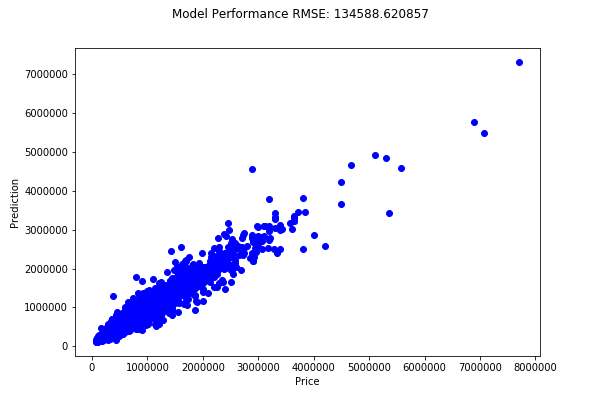
To measure the success of this model, the RegressionEvaluator function calculates the RMSE of the model predictions. To further understand our new model, we also visualize the predictions for the entire dataset using the matplotlib package.

import matplotlib.pyplot as plt

evaluator = RegressionEvaluator(labelCol="label", predictionCol="prediction", metricName="rmse")

rmse = evaluator.evaluate(predictions)

rfPred = cvModel.transform(df)

rfResult = rfPred.toPandas()

plt.plot(rfResult.label, rfResult.prediction, 'bo')
plt.xlabel('Price')
plt.ylabel('Prediction')
plt.suptitle("Model Performance RMSE: %f" % rmse)
plt.show()

Our modeling was fruitful! We beat our baseline by a factor of 1.7. Also, we can see that our predictions are clustered around the diagonal which indicates the model has established predictive significance within the features.

FEATURE IMPORTANCE

Interpretability is very important in machine learning. Non-technical stakeholders are rarely satisfied with predictions coming from a black box. This compels machine learning practitioners to understand which features were most important to the outcomes.

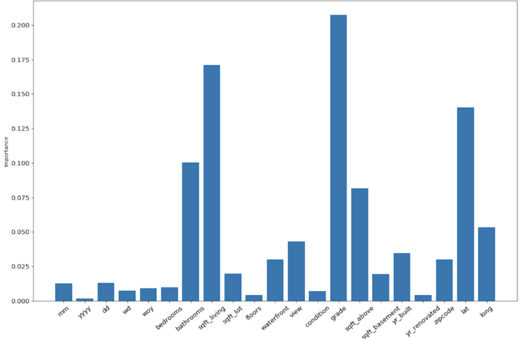
Fortunately, Spark ML accounts for this. The function featureImportances establishes a percentage of how influential each feature is on the model’s predictions.

To isolate the model that performed best in our parameter grid, literally run bestModel. Then, select the Random Forest stage from our pipeline.

bestPipeline = cvModel.bestModel
bestModel = bestPipeline.stages[1]

importances = bestModel.featureImportances

x_values = list(range(len(importances)))

plt.bar(x_values, importances, orientation = 'vertical')
plt.xticks(x_values, feature_list, rotation=40)
plt.ylabel('Importance')
plt.xlabel('Feature')
plt.title('Feature Importances')

It looks like the grade, the square footage, the latitude, and the number of bathrooms are the biggest predictors of the final sale price.

BEST HYPERPARAMETERS

Finally, let’s investigate which parameters performed best. Our ‘Best Model’ object has a series of “get” parameter functions that select out the parameter values which had the highest performance.

print('numTrees - ', bestModel.getNumTrees)
print('maxDepth - ', bestModel.getOrDefault('maxDepth'))

This outputs the following selection from our hyperparameter grid:

• numTrees – 50
• maxDepth – 25

This outcome suggests that our model benefits from growing more trees and allowing the branches to grow deeper.

CONCLUSION

Without much more tuning, it looks like our hypothetical real estate dilettante is able to use predictive guidance for housing prices. Also, knowing the most important features that drive price could be immensely valuable – without ever having to return to our model.

The initial output also serves as a steer if we wanted to continue tuning our model. Which features can we ignore to get better performance? Which parameters should we fix in order to test others?

Spark ML is a very powerful tool for machine learning. This example demonstrates the basic workflow and how to use some of Spark ML’s more compelling features, namely Pipelines and Hyperparameter Grids.

Learn how to spend more time getting insight with Magpie; sign up for a demo.

Brendan Freehart is a Data Engineer at Silectis. 
You can find him on LinkedIn.