Apache Spark: A Beginner’s Guide to Optimizing Spark Scripts

This blog post covers Apache Spark basics and teaches readers why optimizing Spark scripts is important, and how to do it for both memory and runtime efficiency. This blog post is best suited for data analysts and data scientists looking for information on optimizing existing Spark workflows or creating new ones.

INTRODUCTION: WHAT IS APACHE SPARK?

Apache Spark is an open-sourced distributed compute framework, which provides users with lightning-fast analytics for big data processing. Coupled with its speed, Spark is also built to distribute data processing tasks across multiple computers.  These two capabilities are the building blocks for continued success as businesses reach for new technological advantages to help their big data and analytics teams search through massive data stores to find insight.

In order to leverage Spark’s capabilities, users need a compute cluster and a solid understanding of Spark infrastructure, job submission parameters, and scripting syntax. In order to begin writing Spark scripts, users typically need to know either Scala or Python. On top of that, without proper infrastructure maintenance, users can rack up quite a bill on compute resources. All of these factors make Apache Spark difficult to leverage effectively without an experienced team of engineers.

Silectis built the Magpie platform on top of Apache Spark to provide a user-friendly way of leveraging distributed compute resources without the overhead of deploying and maintaining a Spark cluster or even learning a functional programming language like Python or Scala. While prior knowledge of Spark’s inner-workings is certainly not required to effectively use Magpie, some Spark tuning knowledge can help users create more efficient ETL workflows. In this blog post, we will go over ways to get the most out of Spark’s compute capacity to minimize resource allocation and runtimes.

HOW DOES APACHE SPARK WORK?

In order to understand how to optimize Spark scripts and workflows, it is important to first understand Spark at a high level. Apache Spark was built using a manager/worker architecture, where a single driver or manager node distributes compute tasks to a number of executors which live within worker nodes. One of the primary advantages that this architecture allows is parallel processing or parallelism.

PARALLELISM

A real-world metaphor of Spark parallelism can be illustrated through a teacher grading a stack of quizzes for their class. The teacher could go through each quiz and grade them on their own. This will take t*n time where t is the amount of time that it takes to grade one quiz and n is the number of quizzes. This method involves no parallelism and can be compared to processing data using the Pandas Python library or other non-distributed processing engines. The other faster option is for the teacher to distribute the quizzes to several students and have them grade the papers. Given the teacher has distributed the quizzes evenly, we will see perfect parallelism in the grading of the quizzes and it will take t*n/s time where s is the number of helpers. In this example, the teacher can be viewed as the Spark Driver or Manager and the students helping to grade quizzes can be viewed as the Executors. The distribution of the one original stack of quizzes into s smaller stacks of quizzes can be viewed as an example of partitioning data.

Now that we’ve learned about parallelism, let’s move on to a messier topic… Shuffling.     

SPARK SHUFFLING

In Spark, shuffling can be defined as the process of moving data amongst partitions. Shuffling is extremely expensive in terms of both time and memory utilization. While unnecessary shuffling operations should be avoided especially in operational workflows, they are often critical to the completion of different data transformations. Below are a few common operations that require expensive shuffles:

• JOIN
• GROUP BY
• ORDER BY

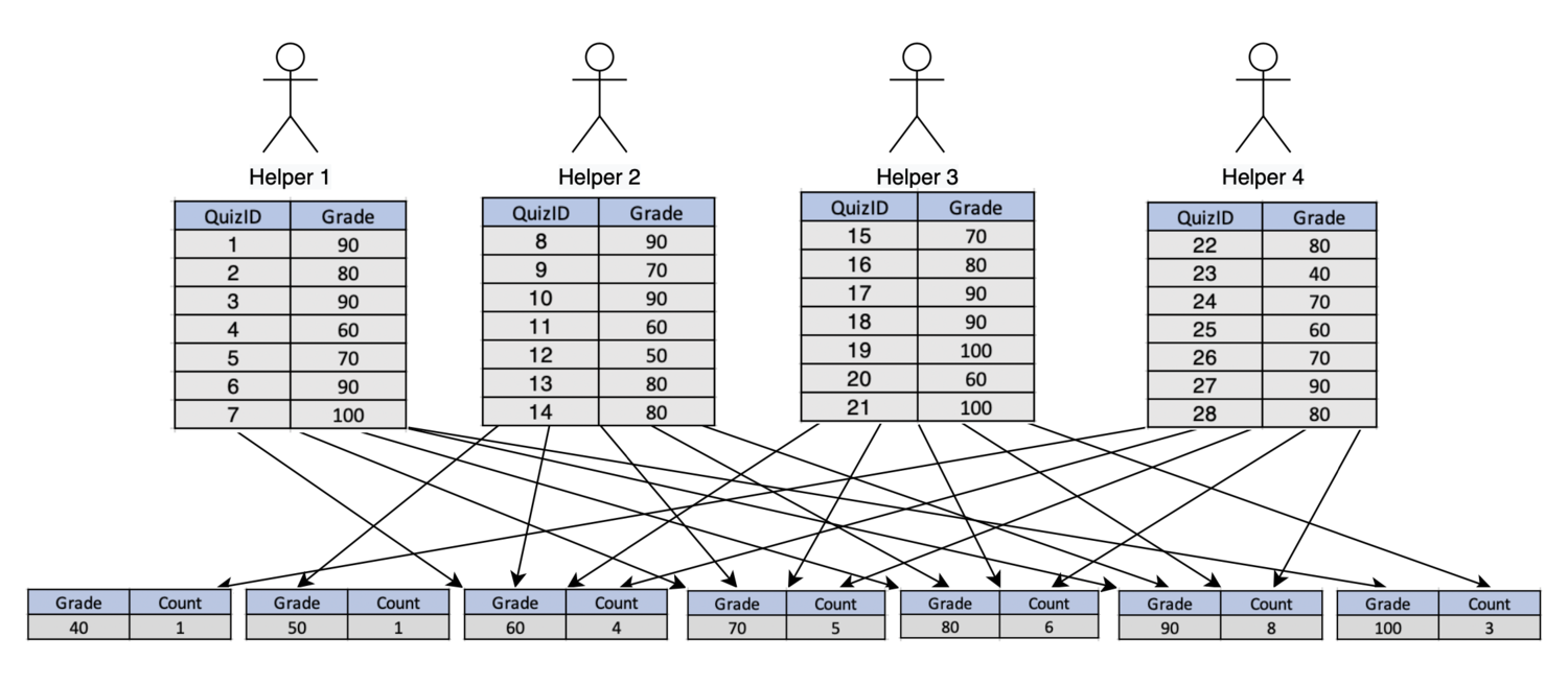
To conceptualize shuffling, let’s continue with our previous metaphor. Now that the students have graded all of the quizzes, the teacher wants to set a curve for the quiz scores. To do this, the teacher tells the helpers to get a COUNT(score) from the quizzes, GROUP BY GRADE. This effectively tells the helpers to create stacks of quizzes by grade and then count each stack. Stop to think about how this will be accomplished. You probably imagine students sending all quizzes of the same grade into a new stack dedicated to the corresponding grade. It should look something like what you see depicted below:

Remember each of the resulting blocks can be considered a new partition, which must also live within executor memory. That means, each arrow represents data shuffling or “moving amongst partitions”. While we’re able to put this into a relatively straight-forward diagram at this small metaphorical scale, it is easy to see how shuffling can become extremely complex as the size of our datasets grow.

MINIMIZING SHUFFLING/MAXIMIZING PARALLELISM

Now it’s time to learn how to tune or optimize Spark scripts with parallelism and shuffling in mind. In this section we’ll cover how users can begin optimizing Spark workflows through the use of broadcast joins, repartitioning, and filtering. Let’s start by talking about minimizing shuffling on join commands. 

To illustrate this, we’ll use an example:

HYPOTHETICAL USE CASE

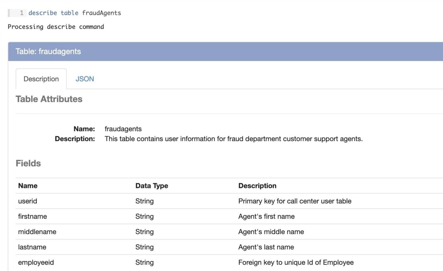
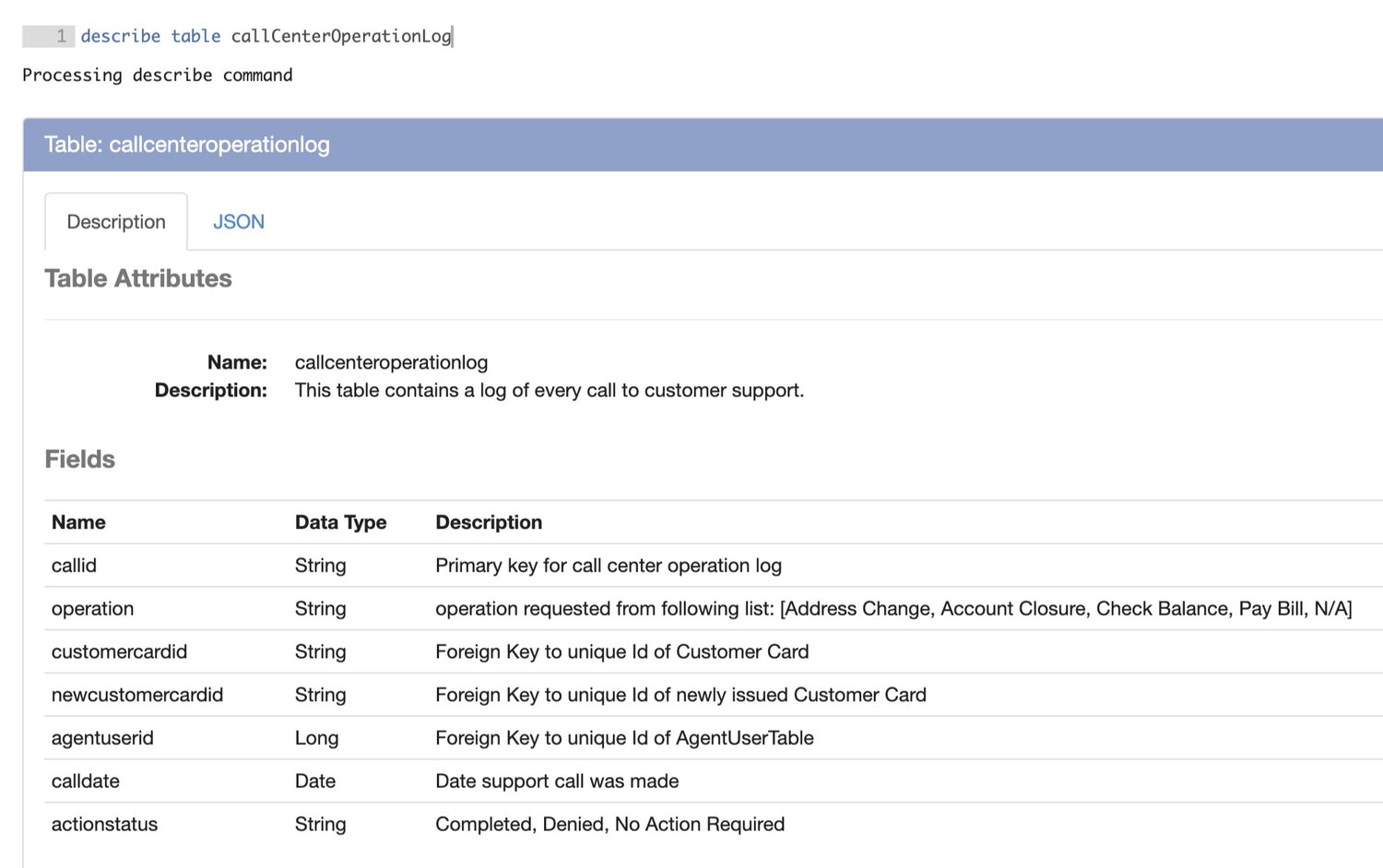
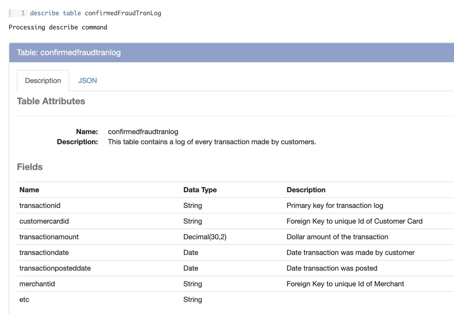
In this scenario we are a credit card company hoping to identify call center agents who are frequently approving fraudulent address change requests. In order to do this we will use 3 datasets, which we will assume are parquet files that have been loaded into our data engineering platform, Magpie. All code will be executed in the Magpie notebook using SQL-like syntax. The datasets are described below through Magpie’s describe table command:

Now that we’ve taken a look at our datasets and understand their schemas let’s begin our transformations. The first major transformation will be combining the Call Center Operation Log and the Agent User Table into a temporary table containing the following fields:

• agentUserId, firstName, middleName, lastName, employeeId, callId, operation, customerCardId, newCustomerCardId, agentUserId, callDate, actionStatus

This will require using an INNER JOIN between the two tables on the following condition:

callcenteroperationlog.agentuserid = fraudagents.userid

Before any resource-intensive transformations like joins, we should consider ways to minimize the size of the datasets. Often times this can be done through simple filtering operations. In this case, we are only trying to analyze “Address Change” requests with the status “Completed”; so let’s filter on those elements through the following command:

create temp table filtered_operation_log from sql( 
SELECT * 
FROM callCenterOperationLog 
WHERE operation = 'Address Change' and actionstatus = 'Completed'
)

For the purposes of this exercise we’ll estimate that completed address change requests account for roughly 10% of call center operations. That means the size of the filtered operation log temporary table is now ~10MB in size. The next thing we can observe is the size difference between our filtered temporary table and the Agent User Table (10MB vs <1MB). When performing join operations on tables or dataframes of drastically different sizes, we should always consider using Spark’s broadcast join feature.

BROADCAST JOINS

In Spark, the broadcast operation is used to push a dataset into memory on every individual executor. When executing a broadcast join, Spark is able to maintain the parallelism of the larger dataset and eliminate the need for shuffling between executors. In order to execute a broadcast join the smaller dataset must be small enough to fit within the allotted executor memory with plenty of room to spare. When consuming datasets of somewhat unpredictable size, explicitly invoking a broadcast join can result in out of memory errors. Fortunately, Spark has an autoBroadcastJoinThreshold parameter which can be used to avoid this risk. By default Spark uses 1GB of executor memory and 10MB as the autoBroadcastJoinThreshold. This means Spark will automatically use a broadcast join to complete join operations when one of the datasets is smaller than 10MB. 

To illustrate a broadcast join through our initial metaphor, consider the grading process. The teacher (driver) has tasked the helpers (executors) with grading each quiz. Grading is done by joining the quiz results with an answer sheet. The standard Spark join would partition the answer sheet and distribute pieces of it to each helper. Then, the helpers would need to shuffle the pieces of the answer sheet amongst each other, comparing the quizzes in their possession to each piece of the answer sheet separately. This is obviously not going to be very efficient. Instead, since the answer sheet is very small, it makes more sense to make a copy of the answer sheet for each helper and broadcast the answer sheet to them. Then, each helper can compare the quizzes to their copy of the answer sheet without any shuffling or communicating between the other helpers.

BACK TO THE USE CASE

Now that you know what a broadcast join is, let’s apply this concept in our join of the Call Center Operation Log and the Fraud Agent User Table. Since the Spark’s default autoBroadcastJoinThreshold is 10MB, we know that Spark will execute a broadcast join by default through the Magpie SQL command below:

create temp table call_center_table from sql( 
SELECT * 
FROM filtered_operation_log as ops 
INNER JOIN fraudagents as agents ON ops.agentuserid = agents.userid
)

Through these simple transformations we have been able to shrink the amount of operation log data by 90% and eliminate shuffling from our join!

Now that the temporary Call Center Table has been created, it is time to join this data with the Confirmed Fraud Transaction log. The first thing to notice about this join is how wide the file is. It contains 20 columns, most of which we will not need in our output. Prior to our first join, we used the ‘where’ command to complete a row-wise filter. This time we will use the ‘select’ command to complete a column-wise filter.

create temp table filtered_fraud_transactions from sql( 
SELECT transactionid, customercardid, transactionamount, transactiondate 
FROM confirmedFraudTranLog
)

After filtering this table we’ve removed 16 out of the 20 columns. Assuming each column takes up the same amount of memory we can estimate the previously 40GB dataset to be approximately 8GB. Even after filtering the partitions the resulting table is extremely large relative to our Call Center Table. Assuming our executors are large enough, we’ll want to execute another broadcast join. Before that though, let’s explore repartitioning.

REPARTITIONING

By repartitioning we can speed up joins and other operations by increasing the amount of parallelism we are able to achieve. In this scenario our source data is partitioned on the column transactionPostedDate, so depending on the number of transactions posted on a given day, partitions may vary greatly in size. For instance, on Black Friday transaction volume increases dramatically. Our partition sizes for that day can be expected to increase at the same rate. In this case, the executors in charge of processing the Black Friday partitions would take much longer to complete their tasks, leaving finished executors waiting. This is a great scenario to consider repartitioning. By evening out our partition sizes we’ll be able to achieve greater parallelism.

When repartitioning we’ll want to consider the number of partitions we want. This is generally based on the number of cores in the cluster, the size of the dataset under evaluation, and the complexity of the transformations to be run. It is best to repartition to some multiple of the number of cores in the cluster. In this case, let’s say there are 5 cores per executor and 20 executors in the cluster making 100 total cores. Since we are dealing with a relatively large dataset and will be executing a complex transformation, we’ll want to use many partitions. Let’s go with 5*total cores, or 500.123save table filtered_fraud_transactions as temp table repartitioned_fraud_transactions with partitions 500

After repartitioning this data we can execute a broadcast join knowing that the shuffling has been minimized and the parallelism has been optimized. But, before we execute the JOIN we most evaluate the size of our datasets to ensure that the broadcast join will in fact be executed. The call_center_table took a 10MB dataset and joined it with a dataset that was ~1MB. Due to the fact that each record of the Filtered Operation Log dataset was associated with a userId from the Fraud Agents Table, we know that the resulting dataset had the same record count as the Filtered Operation Log. We also know that the resulting call_center_table inherited the columns from the Fraud Agents Table as well making it 5 columns wider. Assuming that each column is the same size in memory, we can estimate that call_center_table is slightly under two times the size of the Filtered Operation Log. This exceeds Spark’s default, so we’ll need to bump up the autoBroadCastJoinThreshold to 20MB in order to make use of the broadcast join feature in our SQL statement. The next step is executed through the following commands:

%sql
SET spark.sql.autoBroadcastJoinThreshold = 20,971,520 -- 20MB

create temp table agent_associated_fraud_transactions from sql( 
SELECT trxn.customercardid, cc.agentuserid 
FROM repartitioned_fraud_transactions as trxn 
INNER JOIN call_center_table as cc ON trxn.customercardid = cc.newcustomercardid
)

From this result we can perform some analytical operations to gain the insights we are looking for. To do this we will GROUP BY agentUserId and then aggregate on the number of distinct customerCardIds through the following command:

%sql
SELECT agentuserid, COUNT(DISTINCT customercardid) 
FROM agent_associated_fraud_transactions 
GROUP BY agentuserid;

The resulting table will display the number of Address Change requests which resulted in fraud transactions for each Agent.

Through this use case we were able to demonstrate how Mapgie is able to help users facilitate complex data transformations, while touching on key Spark tuning topics like broadcast joining, repartitioning, and filtering.

CONCLUSION

In this post we explored several fundamental Apache Spark concepts and discuss techniques on optimizing spark scripts to help you get more out of your Spark jobs. Hopefully this post has equipped you with the knowledge and context needed to optimize your existing Spark workflows and swiftly create new ones.

If your organization wants to set up advanced data pipelines without the hassle of managing infrastructure, you can learn more about Magpie by scheduling a demo.

If you’re interested in solving today’s big data challenges, apply for one of our open positions on our careers page.